[pytorch] MNIST 예제

기존 텐서플로로 공부를 해왔다. 그런데 최근 트렌드가 텐서플로에서 파이토치로 많이 넘어간다고 한다. 

파이썬과 많이 비슷하며 연구진들이 정말 많이 사용해 논문 같은 예시 코드가 파이토치로 많이 구현되있어서 이왕 제대로 각잡고 공부하는거 토치를 한 번 공부해 보려고 한다.

실제로 간단한 기본 MNIST를 하면서 느낀점은 ... 

더 어렵다. 확실히 더 어렵다... 아직 잘 몰라서 이런 말 하기도 조심스럽지만 텐서플로 같은 경우에는 모델을 돌릴 때 아주 간단하게 돌릴 수 있었다. 하지만 디테일하게 들어가서 구조를 들여다 보고 모델이 돌아가는 방식을 살피기는 쉽지 않았다. 그냥 필요한 값만 넣어주면 알아서 돌아가는 시스템이였다.

근데 파이토치는 모델의 구조 순서에 따라 직접 구성하는 방식이고 원리를 잘 이해한 상태라면 그냥 그 원리 그대로가 반영 되있는 느낌이였다. 그리고 파이썬에 가깝다는 말도 대충 무슨 말인지 알 것 같았다

일단은 예제 이기 때문에 코드와 결과만 설명하고 넘어가겠다.

 

import torch
is_cuda = torch.cuda.is_available()
device = torch.device('cuda' if is_cuda else 'cpu')
print(device)
import torch.nn as nn #딥러닝 네트워크의 기본 구성요소
import torch.nn.functional as F # 딥러닝에 자주 쓰는 함수를 F로 불러오겠다
import torch.optim as optim # 가중치 추정에 필요한 최적화 알고리즘을 포함한 모듈을 optim으로 지정
from torchvision import datasets, transforms #torchvision에서 데이터셋과 transform을 가져온다

from matplotlib import pyplot as plt
%matplotlib inline

HyperParameter 지정

batch_size = 50
epoch_num = 15
learning_rate = 0.0001

train_data = datasets.MNIST(root = './data', train = True, download = True, transform = transforms.ToTensor())
test_data = datasets.MNIST(root = './data', train = False, transform = transforms.ToTensor())
# transform : MNIST 저장과 동시에 전처리를 할 수 있는 옵션. 이미지를 텐서로 변형하는 전처리여서 ToTensor()를 써준다.

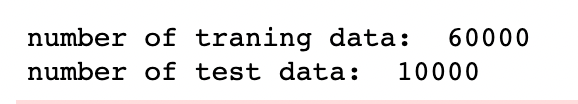
print('number of traning data: ', len(train_data))
print('number of test data: ', len(test_data))

root = ./data (현재 디텍토리에 data라는 폴더를 만들어서 저장하겠다.) 

transforms.ToTensor() : 이미지를 받음으로 동시에 tensor로 받는 전처리를 하는 것이다.

image, label = train_data[0]     # image 와 label 을 받아온다.

# MNIST는 단일 채널로 [1,28,28] 3차원 텐서이다. 3차원 텐서를 2차원으로 줄이기 위해 image.squeeze()를 사용한다.
plt.imshow(image.squeeze().numpy(), cmap = 'gray') #squeeze() : 크기가 1인 차원을 없애는 함수로 2차원 [28,28]로  만든다.
plt.title('label : %s' % label)
plt.show()

[미니 배치 구성하기]

 

# DataLoader는 손쉽게 배치를 구성하며 학습과정을 반복 시행 할때 마다 미니배치를 불러오는 유용한 함수
train_loader = torch.utils.data.DataLoader(dataset = train_data,
                                          batch_size = batch_size,
                                          shuffle = True)
test_loader = torch.utils.data.DataLoader(dataset = test_data,
                                          batch_size = batch_size,
                                          shuffle = True)


first_batch = train_loader.__iter__().__next__()
print('{:15s} | {:<25s} | {}'.format('name', 'type', 'size'))
print('{:15s} | {:<25s} | {}'.format('Num of Batch', '',
                                     len(train_loader)))
print('{:15s} | {:<25s} | {}'.format('first_batch', str(type(first_batch)),
                                    len(first_batch)))
print('{:15s} | {:<25s} | {}'.format('first_batch[0]',
                                    str(type(first_batch[0])),
                                    first_batch[0].shape))
print('{:15s} | {:<25s} | {}'.format('first_batch[1]',
                                    str(type(first_batch[1])),
                                    first_batch[1].shape))

[CNN 구조 설계하기]

class CNN(nn.Module):
    def __init__(self): #모델에 사용되는 가중치를 정의
        super(CNN,self).__init__() #super()를 통해 nn.Module 클래스의 속성을 상속 받고 초기화
        self.conv1 = nn.Conv2d(1,32,3,1)   #in_channel / out_channel / kernel_size / stride
        self.conv2 = nn.Conv2d(32, 64, 3, 1)
        self.dropout1 = nn.Dropout2d(0.25)   # 0.25 확률의 드랍아웃을 지정
        self.dropout2 = nn.Dropout2d(0.5)
        self.fc1 = nn.Linear(9216,128)   # 9264 -> 128 -> 10
        self.fc2 = nn.Linear(128,10)
    
    def forward(self,x) :  # 입력이미지와 정의한 가중치를 이용해 feed forward 계산
        x = self.conv1(x)
        x = F.relu(x)
        x = self.conv2(x)
        x = F.relu(x)
        x = F.max_pool2d(x,2)     # (2x2 크기의 필터로 맥스 풀링 한다. 이건 가중치 할 필요가 없어서 위에서 정의 안했다)
        x = self.dropout1(x)
        x = torch.flatten(x,1)
        x = self.fc1(x)
        x = F.relu(x)
        x = self.dropout2(x)
        x = self.fc2(x)
        output = F.log_softmax(x, dim=1) #softmax 말고 log_softmax()를 쓰면 연산속도를 올릴 수 있다.
        return output

구조를 그림으로 그리면

[ 모델 최적화]

model = CNN().to(device)
optimizer = optim.Adam(model.parameters(), lr = learning_rate)
criterion = nn.CrossEntropyLoss()    # 손실함수로 크로스엔트로피

[모델 학습]

model.train()
i = 0
for epoch in range(epoch_num):
    for data, target in train_loader:
        data = data.to(device)
        target = target.to(device)
        optimizer.zero_grad()
        output = model(data)
        loss = criterion(output, target) # 계산값과 결과값에 대해 손실을 구해보자
        loss.backward()
        optimizer.step()  # 역전파로 계산해서 모델 가중치 업데이트
        if i % 1000 == 0 :
            print('Train Step : {}\tLoss: {:.3f}'. format(i, loss.item()))
        i += 1

 

[모델 평가]

model.eval()
correct = 0
for data, target in test_loader:
    data = data.to(device)
    target = target.to(device)
    output = model(data)
    prediction = output.data.max(1)[1]
    correct += prediction.eq(target.data).sum()
    
print('Test set: Accuracy : {:.2f}%'.format(100 * correct / len(test_loader.dataset)))

 

정확도 99.09 % 가 나왔다.

 

이게 너무 잘 정형화된 사기 데이터여서 당연히 이런 결과가 나온다고 한다. 

파이토치에 빨리익숙해지고 싶다.